Modeling

Introduction

MuJoCo can load XML model files in its native MJCF format, as well as in the popular but more limited URDF format. This chapter is the MJCF modeling guide. The reference manual is available in the XML Reference chapter. The URDF documentation can be found elsewhere; here we only describe MuJoCo-specific URDF extensions.

MJCF models can represent complex dynamical systems with a wide range of features and model elements. Accessing all these features requires a rich modeling format, which can become cumbersome if it is not designed with usability in mind. Therefore we have made an effort to design MJCF as a scalable format, allowing users to start small and build more detailed models later. Particularly helpful in this regard is the extensive default setting mechanism inspired by the idea of Cascading Style Sheets (CSS) inlined in HTML. It enables users to rapidly create new models and experiment with them. Experimentation is further aided by numerous options which can be used to reconfigure the simulation pipeline, and by quick re-loading that makes model editing an interactive process.

One can think of MJCF as a hybrid between a modeling format and a programming language. There is a built-in compiler, which is a concept normally associated with programming languages. While MJCF does not have the power of a general-purpose programming language, a number of sophisticated compile-time computations are invoked automatically depending on how the model is designed.

Loading models

As explained in Model instances in the Overview chapter, MuJoCo models can be loaded from plain-text XML files in the MJCF or URDF formats, and then compiled into a low-level mjModel. Alternatively a previously saved mjModel can be loaded directly from a binary MJB file - whose format is not documented but is essentially a copy of the mjModel memory buffer. MJCF and URDF files are loaded with mj_loadXML while MJB files are loaded with mj_loadModel.

When an XML file is loaded, it is first parsed into a document object model (DOM) using the TinyXML parser internally. This DOM is then processed and converted into a high-level mjCModel object. The conversion depends on the model format - which is inferred from the top-level element in the XML file, and not from the file extension. Recall that a valid XML file has a unique top-level element. This element must be mujoco for MJCF, and robot for URDF.

Compiling models

Once a high-level mjCModel is created - by loading an MJCF file or a URDF file, or programmatically when such functionality becomes available - it is compiled into mjModel. Even though loading and compilation are presently combined in one step, compilation is independent of loading, meaning that the compiler works in the same way regardless of how mjCModel was created. Both the parser and the compiler perform extensive error checking, and abort when the first error is encountered. The resulting error messages contain the row and column number in the XML file, and are self-explanatory so we do not document them here. The parser uses a custom schema to make sure that the file structure, elements and attributes are valid. The compiler then applies many additional semantic checks. Finally, one simulation step of the compiled model is performed and any runtime errors are intercepted. The latter is done by (temporarily) setting mju_user_error to point to a function that throws C++ exceptions; the user can implement similar error-interception functionality at runtime if desired.

The entire process of parsing and compilation is very fast - less than a second if the model does not contain large meshes or actuator lengthranges that need to be computed via simulation. This makes it possible to design models interactively, by re-loading often and visualizing the changes. Note that the simulate.cc code sample has a keyboard shortcut for re-loading the current model (Ctrl+L).

Saving models

An MJCF model can consist of multiple (included) XML files as well as meshes, height fields and textures referenced from the XML. After compilation, the contents of all these files are assembled into mjModel, which can be saved into a binary MJB file with mj_saveModel. The MJB is a stand-alone file and does not refer to any other files. It also loads faster. So we recommend saving commonly used models as MJB and loading them when needed for simulation.

It is also possible to save a compiled mjCModel as MJCF with mj_saveLastXML. If any real-valued fields in the corresponding mjModel were modified after compilation (which is unusual but can happen in system identification applications for example), the modifications are automatically copied back into mjCModel before saving. Note that structural changes cannot be made in the compiled model. The XML writer attempts to generate the smallest MJCF file which is guaranteed to compile into the same model, modulo negligible numeric differences caused by the plain text representation of real values. The resulting file may not have the same structure as the original because MJCF has many user convenience features, allowing the same model to be specified in different ways. The XML writer uses a “canonical” subset of MJCF where all coordinates are local and all body positions, orientations and inertial properties are explicitly specified. In the Computation chapter we showed an example MJCF file and the corresponding saved example.

MJCF Mechanisms

MJCF uses several mechanisms for model creation which span multiple model elements. To avoid repetition we describe them in detail only once in this section. These mechanisms do not correspond to new simulation concepts beyond those introduced in the Computation chapter. Their role is to simplify the creation of MJCF models, and to enable the use of different data formats without need for manual conversion to a canonical format.

Kinematic tree

The main part of the MJCF file is an XML tree created by nested body elements. The top-level body is special and is called worldbody. This tree organization is in contrast with URDF where one creates a collection of links and then connects them with joints that specify a child and a parent link. In MJCF the child body is literally a child of the parent body, in the sense of XML.

When a joint is defined inside a body, its function is not to connect the parent and child but rather to create motion degrees of freedom between them. If no joints are defined within a given body, that body is welded to its parent. A body in MJCF can contain multiple joints, thus there is no need to introduce dummy bodies for creating composite joints. Instead simply define all the primitive joints that form the desired composite joint within the same body. For example, two sliders and one hinge can be used to model a body moving in a plane.

Other MJCF elements can be defined within the tree created by nested body elements, in particular joint, geom, site, camera, light. When an element is defined within a body, it is fixed to the local frame of that body and always moves with it. Elements that refer to multiple bodies, or do not refer to bodies at all, are defined in separate sections outside the kinematic tree.

Default settings

MJCF has an elaborate mechanism for setting default attribute values. This allows us to have a large number of elements and attributes needed to expose the rich functionality of the software, and at the same time write short and readable model files. This mechanism further enables the user to introduce a change in one place and have it propagate throughout the model. We start with an example.

<mujoco>
    <default class="main">
        <geom rgba="1 0 0 1"/>
        <default class="sub">
            <geom rgba="0 1 0 1"/>
        </default>
    </default>

    <worldbody>
        <geom type="box"/>
        <body childclass="sub">
            <geom type="ellipsoid"/>
            <geom type="sphere" rgba="0 0 1 1"/>
            <geom type="cylinder" class="main"/>
        </body>
    </worldbody>
</mujoco>

This example will not actually compile because some required information is missing, but here we are only interested in the setting of geom rgba values. The four geoms created above will end up with the following rgba values as a result of the default setting mechanism:

geom type	geom rgba
box	1 0 0 1
ellipsoid	0 1 0 1
sphere	0 0 1 1
cylinder	1 0 0 1

The box uses the top-level defaults class “main” to set the values of its undefined attributes, because no other class was specified. The body specifies childclass “sub”, causing all children of this body (and all their children etc.) to use class “sub” unless specified otherwise. So the ellipsoid uses class “sub”. The sphere has explicitly defined rgba which overrides the default settings. The cylinder specifies defaults class “main”, and so it uses “main” instead of “sub”, even though the latter was specified in the childclass attribute of the body containing the geom.

Now we describe the general rules. MuJoCo supports unlimited number of defaults classes, created by possibly nested default elements in the XML. Each class has a unique name - which is a required attribute except for the top-level class whose name is “main” if left undefined. Each class also has a complete collection of dummy model elements, with their attributes set as follows. When a defaults class is defined within another defaults class, the child automatically inherits all attribute values from the parent. It can then override some or all of them by defining the corresponding attributes. The top-level defaults class does not have a parent, and so its attributes are initialized to internal defaults which are shown in the Reference chapter.

The dummy elements contained in the defaults classes are not part of the model; they are only used to initialize the attribute values of the actual model elements. When an actual element is first created, all its attributes are copied from the corresponding dummy element in the defaults class that is currently active. There is always an active defaults class, which can be determined in one of three ways. If no class is specified in the present element or any of its ancestor bodies, the top-level class is used (regardless of whether it is called “main” or something else). If no class is specified in the present element but one or more of its ancestor bodies specify a childclass, then the childclass from the nearest ancestor body is used. If the present element specifies a class, that class is used regardless of any childclass attributes in its ancestor bodies.

Some attributes, such as body inertia, can be in a special undefined state. This instructs the compiler to infer the corresponding value from other information, in this case the inertias of the geoms attached to the body. The undefined state cannot be entered in the XML file. Therefore once an attribute is defined in a given class, it cannot be undefined in that class or in any of its child classes. So if the goal is to leave a certain attribute undefined in a given model element, it must be undefined in the active defaults class.

A final twist here is actuators. They are different because some of the actuator-related elements are actually shortcuts, and shortcuts interact with the defaults setting mechanism in a non-obvious way. This is explained in the Actuator shortcuts section below.

Coordinate frames

The positions and orientations of all elements defined in the kinematic tree are expressed in local coordinates, relative to the parent body for bodies, and relative to the body that contains the element for geoms, joints, sites, cameras and lights.

A related attribute is compiler/angle. It specifies whether angles in the MJCF file are expressed in degrees or radians (after compilation, angles are always expressed in radians).

Positions are specified using

pos: real(3), “0 0 0”

Position relative to parent.

Frame orientations

Several model elements have right-handed spatial frames associated with them. These are all the elements defined in the kinematic tree except for joints. A spatial frame is defined by its position and orientation. Specifying 3D positions is straightforward, but specifying 3D orientations can be challenging. This is why MJCF provides several alternative mechanisms. No matter which mechanism the user chooses, the frame orientation is always converted internally to a unit quaternion. Recall that a 3D rotation by angle \(a\) around axis given by the unit vector \((x, y, z)\) corresponds to the quaternion \((\cos(a/2), \: \sin(a/2) \cdot (x, y, z))\). Also recall that every 3D orientation can be uniquely specified by a single 3D rotation by some angle around some axis.

All MJCF elements that have spatial frames allow the five attributes listed below. The frame orientation is specified using at most one of these attributes. The quat attribute has a default value corresponding to the null rotation, while the others are initialized in the special undefined state. Thus if none of these attributes are specified by the user, the frame is not rotated.

quat: real(4), “1 0 0 0”

If the quaternion is known, this is the preferred was to specify the frame orientation because it does not involve conversions. Instead it is normalized to unit length and copied into mjModel during compilation. When a model is saved as MJCF, all frame orientations are expressed as quaternions using this attribute.

axisangle: real(4), optional

These are the quantities \((x, y, z, a)\) mentioned above. The last number is the angle of rotation, in degrees or radians as specified by the angle attribute of compiler. The first three numbers determine a 3D vector which is the rotation axis. This vector is normalized to unit length during compilation, so the user can specify a vector of any non-zero length. Keep in mind that the rotation is right-handed; if the direction of the vector \((x, y, z)\) is reversed this will result in the opposite rotation. Changing the sign of \(a\) can also be used to specify the opposite rotation.

euler: real(3), optional

Rotation angles around three coordinate axes. The sequence of axes around which these rotations are applied is determined by the eulerseq attribute of compiler and is the same for the entire model.

xyaxes: real(6), optional

The first 3 numbers are the X axis of the frame. The next 3 numbers are the Y axis of the frame, which is automatically made orthogonal to the X axis. The Z axis is then defined as the cross-product of the X and Y axes.

zaxis: real(3), optional

The Z axis of the frame. The compiler finds the minimal rotation that maps the vector \((0, 0, 1)\) into the vector specified here. This determines the X and Y axes of the frame implicitly. This is useful for geoms with rotational symmetry around the Z axis, as well as lights - which are oriented along the Z axis of their frame.

Solver parameters

The solver Parameters section of the Computation chapter explained the mathematical and algorithmic meaning of the quantities \(d, b, k\) which determine the behavior of the constraints in MuJoCo. Here we explain how to set them. Setting is done indirectly, through the attributes solref and solimp which are available in all MJCF elements involving constraints. These parameters can be adjusted per constraint, or per defaults class, or left undefined – in which case MuJoCo uses the internal defaults shown below. Note also the override mechanism available in option; it can be used to change all contact-related solver parameters at runtime, so as to experiment interactively with parameter settings or implement continuation methods for numerical optimization.

Here we focus on a single scalar constraint. Using slightly different notation from the Computation chapter, let \(\ac\) denote the acceleration, \(v\) the velocity, \(r\) the position or residual (defined as 0 in friction dimensions), \(k\) and \(b\) the stiffness and damping of the virtual spring used to define the reference acceleration \(\ar = -b v - k r\). Let \(d\) be the constraint impedance, and \(\au\) the acceleration in the absence of constraint force. Our earlier analysis revealed that the dynamics in constraint space are approximately

(1)\[\ac + d \cdot (b v + k r) = (1 - d)\cdot \au \]

Again, the parameters that are under the user’s control are \(d, b, k\). The remaining quantities are functions of the system state and are computed automatically at each time step.

Impedance

We begin by explaining the constraint impedance \(d\).

Intuitive description of the impedance

The impedance \(d \in (0, 1)\) corresponds to a constraint’s ability to generate force. Small values of \(d\) correspond to weak constraints while large values of \(d\) correspond to strong constraints. The impedance affects the constraint at all times, in particular when the system is at rest. Impedance is set using the solimp attribute.

Recall that \(d\) must lie between 0 and 1; internally MuJoCo clamps it to the range [mjMINIMP mjMAXIMP] which is currently set to [0.0001 0.9999]. It causes the solver to interpolate between the unforced acceleration \(\au\) and reference acceleration \(\ar\). The user can set \(d\) to a constant, or take advantage of its interpolating property and make it position-dependent, i.e., a function of the constraint violation \(r\). Position-dependent impedance can be used to model soft contact layers around objects, or define equality constraints that become stronger with larger violation (so as to approximate backlash, for example). The shape of the function \(d(r)\) is determined by the element-specific parameter vector solimp.

solimp : real(5), “0.9 0.95 0.001 0.5 2”

The five numbers (\(d_0\), \(d_\text{width}\), \(\text{width}\), \(\text{midpoint}\), \(\text{power}\)) parameterize \(d(r)\) – the impedance \(d\) as a function of the constraint violation \(r\).

The first 3 values indicate that the impedance will vary smoothly as \(r\) varies from \(0\) to \(\text{width}\):

\[d(0) = d_0, \quad d(\text{width}) = d_\text{width} \]

The 4th and 5th values, \(\text{midpoint}\) and \(\text{power}\), control the shape of the sigmoidal function that interpolates between \(d_0\) and \(d_\text{width}\), as shown in the plots below. The plots show two reflected sigmoids, because the impedance \(d(r)\) depends on the absolute value of \(r\). The \(\text{power}\) (of the polynomial spline used to generate the function) must be 1 or greater. The \(\text{midpoint}\) (specifying the inflection point) must be between 0 and 1, and is expressed in units of \(\text{width}\). Note that when \(\text{power}\) is 1, the function is linear regardless of the \(\text{midpoint}\).

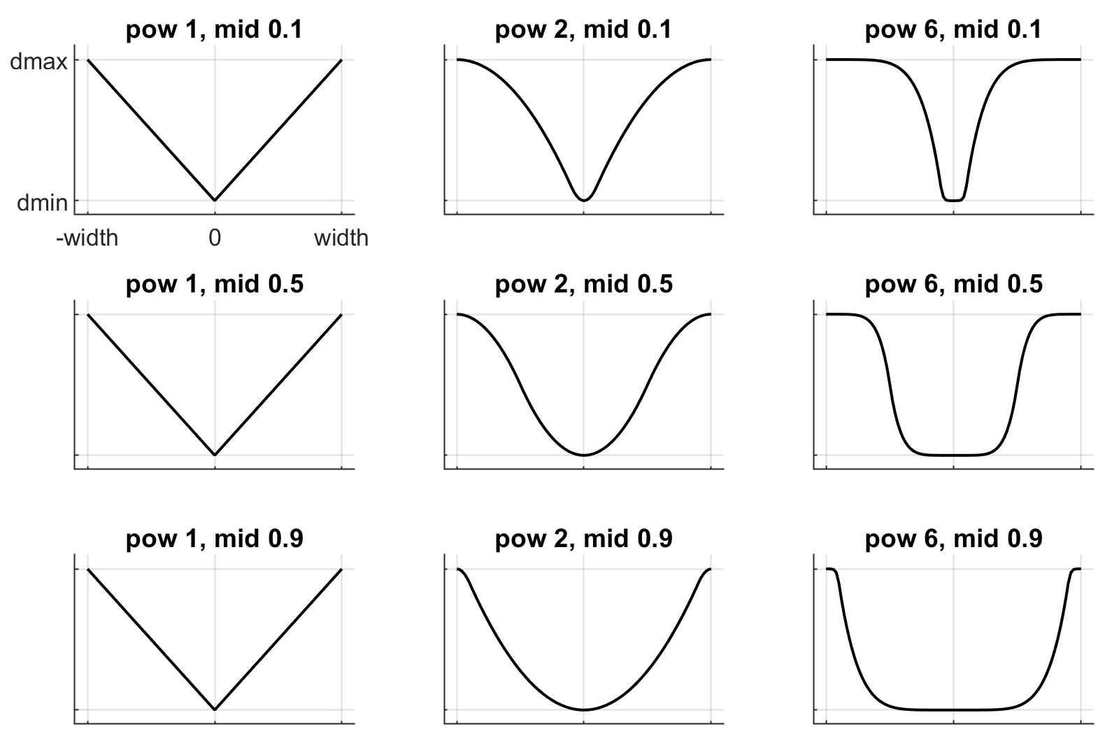
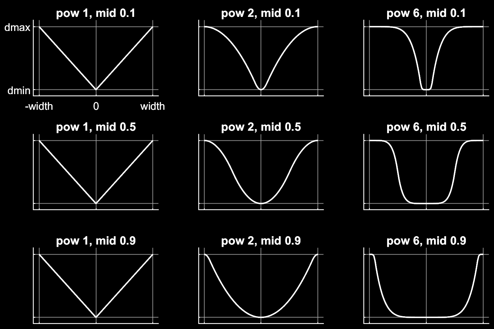
These plots show the impedance \(d(r)\) on the vertical axis, as a function of the constraint violation \(r\) on the horizontal axis.

For equality constraints, \(r\) is the constraint violation. For limits, normal directions of elliptic cones and all directions of pyramidal cones, \(r\) is the (limit or contact) distance minus the margin at which the constraint becomes active; for contacts this margin is margin-gap. Limit and contact constraints are active when \(r < 0\) (penetration).

For friction loss or friction dimensions of elliptic cones, the violation \(r\) is identically zero, so only \(d(0)\) affects these constraints, all other solimp values are ignored.

Tip

For completely smooth dynamics, limits and contacts should have \(d_0=0\).

Reference

Next we explain the setting of the stiffness \(k\) and damping \(b\) which control the reference acceleration \(\ar\).

Intuitive description of the reference acceleration

The reference acceleration \(\ar\) determines the motion that constraint is trying to achieve in order to rectify violation. Imagine a body dropped onto the plane. Upon impact the constraint will generate a normal force which attempts to rectify the penetration using a particular motion; this motion is the reference acceleration.

Another way of understanding the reference acceleration is to think of the unmodeled deformation variables described in the Computation chapter. Imagine two bodies pressed together, leading to deformation at the contact. Now pull the bodies apart very quickly; the motion of the deformation as it settles into its undeformed state is the reference acceleration.

This acceleration is defined by two numbers, a stiffness \(k\) and damping \(b\) which can be set directly or re-parameterized as the time-constant and damping ratio of a mass-spring-damper system (a harmonic oscillator). The reference acceleration is controlled by the solref attribute.

There are two formats for this attribute, determined by the sign of the numbers. If both numbers are positive the specification is considered to be in the \((\text{timeconst}, \text{dampratio})\) format. If negative it is in the “direct” \((-\text{stiffness}, -\text{damping})\) format.

Frictional constraints whose residual is identically 0 have first-order dynamics and the mass-spring-damper analysis below does not apply. In this case the time constant is the rate of exponential decay of the constraint velocity, and the damping ratio is ignored. Equivalently, in the direct format, the \(\text{stiffness}\) is ignored.

solref : real(2), “0.02 1”

We first describe the default, positive-value format where the two numbers are \((\text{timeconst}, \text{dampratio})\).

The idea here is to re-parameterize the model in terms of the time constant and damping ratio of a mass-spring-damper system. By “time constant” we mean the inverse of the natural frequency times the damping ratio. In this case we use a mass-spring-damper model to compute \(k, b\) after suitable scaling. Note that the effective stiffness \(d(r) \cdot k\) and damping \(d(r) \cdot b\) are scaled by the impedance \(d(r)\) which is a function of the distance \(r\). Thus we cannot always achieve the specified mass-spring-damper properties, unless we completely undo the scaling by \(d\). But the latter is undesirable because it would ruin the interpolating property, in particular the limit \(d=0\) would no longer disable the constraint. Instead we scale the stiffness and damping so that the damping ratio remains constant, while the time constant increases when \(d(r)\) gets smaller. The scaling formulas are

\[\begin{aligned} b &= 2 / (d_\text{width}\cdot \text{timeconst}) \\ k &= d(r) / (d_\text{width}^2 \cdot \text{timeconst}^2 \cdot \text{dampratio}^2) \\ \end{aligned} \]

The timeconst parameter should be at least two times larger than the simulation time step, otherwise the system can become too stiff relative to the numerical integrator (especially when Euler integration is used) and the simulation can go unstable. This is enforced internally, unless the refsafe attribute of flag is set to false. The \(\text{dampratio}\) parameter would normally be set to 1, corresponding to critical damping. Smaller values result in under-damped or bouncy constraints, while larger values result in over-damped constraints. Combining the above formula with (1), we can derive the following result. If the reference acceleration is given using the positive number format and the impedance is constant \(d = d_0 = d_\text{width}\), then the penetration depth at rest is

\[r = \au \cdot (1 - d) \cdot \text{timeconst}^2 \cdot \text{dampratio}^2 \]

Next we describe the direct format where the two numbers are \((-\text{stiffness}, -\text{damping})\). This allows direct control over restitution in particular. We still apply some scaling so that the same numbers can be used with different impedances, but the scaling no longer depends on \(r\) and the two numbers no longer interact. The scaling formulas are

\[\begin{aligned} b &= \text{damping} / d_\text{width} \\ k &= \text{stiffness} \cdot d(r) / d_\text{width}^2 \\ \end{aligned} \]

Similarly to the above derivation, if the reference acceleration is given using the negative number format and the impedance is constant, then the penetration depth at rest is

\[r = \frac{\au (1 - d)}{\text{stiffness}} \]

Tip

In the positive-value default format, the \(\text{timeconst}\) parameter controls constraint softness. It is specified in units of time and means “how quickly is the constraint trying to resolve the violation”. Larger values correspond to softer constraints.

The negative-value “direct” format is more flexible, for example allowing for perfectly elastic collisions (\(\text{damping} = 0\)). It is the recommended format for system identification.

A \(\text{dampratio}\) of 1 in the positive-value format is equivalent to \(\text{damping} = 2 \sqrt{ \text{stiffness} }\) in the direct format.

Contact parameters

The parameters of each contact were described in the Contact section of the Computation chapter. Here we explain how these parameters are set. If the geom pair is explicitly defined with the XML element pair, it has attributes specifying all contact parameters directly. In that case the parameters of the individual geoms are ignored. If on the other hand the contact is generated by the dynamic mechanism, its parameters need to be inferred from the two geoms in the contact pair. If the two geoms have identical parameters there is nothing to do, but what if their parameters are different? In that case we use the geom attributes solmix and priority to decide how to combine them. The combination rules for each contact parameter are as follows:

condim

If one of the two geoms has higher priority, its condim is used. If both geoms have the same priority, the maximum of the two condims is used. In this way a frictionless geom and a frictional geom form a frictional contact, unless the frictionless geom has higher priority. The latter is desirable in particle systems for example, where we may not want the particles to stick to any objects.

friction

Recall that contacts can have up to 5 friction coefficients: two tangential, one torsional, two rolling. Each contact in mjData.contact actually has all 5 of them, even if condim is less than 6 and not all coefficients are used. In contrast, geoms have only 3 friction coefficients: tangential (same for both axes), torsional, rolling (same for both axes). Each of these 3D vectors of friction coefficients is expanded into a 5D vector of friction coefficients by replicating the tangetial and rolling components. The contact friction coefficients are then computed according to the following rule: if one of the two geoms has higher priority, its friction coefficients are used. Otherwise the element-wise maximum of each friction coefficient over the two geoms is used. The rationale is similar to taking the maximum over condim: we want the more frictional geom to win. The reason for having 5 coefficients per contact and only 3 per geom is as follows. For a contact pair, we want to allow the most flexible model our solver can handle. As mentioned earlier, anisotropic friction can be exploited to model effects such as skating. This however requires knowing how the two axes of the contact tangent plane are oriented. For a predefined contact pair we know the two geom types in advance, and the corresponding collision function always generates contact frames oriented in the same way - which we do not describe here but it can be seen in the visualizer. For individual geoms however, we do not know which other geoms they might collide with and what their geom types might be, so there is no way to know how the contact tangent plane will be oriented when specifying an individual geom. This is why MuJoCo does not allow anisotropic friction in the individual geom specifications, but only in the explicit contact pair specifications.

margin, gap

The maximum of the two geom margins (or gaps respectively) is used. The geom priority is ignored here, because the margin and gap are distance properties and a one-sided specification makes little sense.

solref, solimp

If one of the two geoms has higher priority, its solref and solimp parameters are used. If both geoms have the same priority, the weighted average is used. The weights are proportional to the solmix attributes, i.e., weight1 = solmix1 / (solmix1 + solmix2) and similarly for weight2. There is one important exception to this weighted averaging rule. If solref for either geom is non-positive, i.e., it relies on the direct format, then the element-wise minimum is used regardless of solmix. This is because averaging solref parameters in different formats would be meaningless.

Contact override

MuJoCo uses an elaborate as well as novel Constraint model described in the Computation chapter. Gaining an intuition for how this model works requires some experimentation. In order to facilitate this process, we provide a mechanism to override some of the solver parameters, without making changes to the actual model. Once the override is disabled, the simulation reverts to the parameters specified in the model. This mechanism can also be used to implement continuation methods in the context of numerical optimization (such as optimal control or state estimation). This is done by allowing contacts to act from a distance in the early phases of optimization - so as to help the optimizer find a gradient and get close to a good solution - and reducing this effect later to make the final solution physically realistic.

The relevant settings here are the override attribute of flag which enables and disables this mechanism, and the o_margin, o_solref, o_solimp attributes of option which specify the new solver parameters. Note that the override applies only to contacts, and not to other types of constraints. In principle there are many real-valued parameters in a MuJoCo model that could benefit from a similar override mechanism. However we had to draw a line somewhere, and contacts are the natural choice because they give rise to the richest yet most difficult-to-tune behavior. Furthermore, contact dynamics often present a challenge in terms of numerical optimization, and experience has shown that continuation over contact parameters can help avoid local minima.

User parameters

A number of MJCF elements have the optional attribute user, which defines a custom element-specific parameter array. This interacts with the corresponding “nuser_XXX” attribute of the size element. If for example we set nuser_geom to 5, then every geom in mjModel will have a custom array of 5 real-valued parameters. These geom- specific parameters are either defined in the MJCF file via the user attribute of geom, or set to 0 by the compiler if this attribute is omitted. The default value of all “nuser_XXX” attributes is -1, which instructs the compiler to automatically set this value to the length of the maximum associated user attribute defined in the model. MuJoCo does not use these parameters in any internal computations; instead they are available for custom computations. The parser allows arrays of arbitrary length in the XML, and the compiler later resizes them to length nuser_XXX.

Some element-specific parameters that are normally used in internal computations can also be used in custom computations. This is done by installing user callbacks which override parts of the simulation pipeline. For example, the general actuator element has attributes dyntype and dynprm. If dyntype is set to “user”, then MuJoCo will call mjcb_act_dyn to compute the actuator dynamics instead of calling its internal function. The user function pointed to by mjcb_act_dyn can interpret the parameters defined in dynprm however it wishes. However the length of this parameter array cannot be changed (unlike the custom arrays described earlier whose length is defined in the MJCF file). The same applies to other callbacks.

In addition to the element-specific user parameters described above, one can include global data in the model via custom elements. For data that change in the course of the simulation, there is also the array mjData.userdata whose size is determined by the nuserdata attribute of the size element.

Solver settings

The computation of constraint forces and constrained accelerations involves solving an optimization problem numerically. MuJoCo has three algorithms for solving this optimization problem: CG, Newton, PGS. Each of them can be applied to a pyramidal or elliptic model of the friction cones, and with dense or sparse constraint Jacobians. In addition, the user can specify the maximum number of iterations, and tolerance level which controls early termination. There is also a second Noslip solver, which is a post-processing step enabled by specifying a positive number of noslip iterations. All these algorithm settings can be specified in the option element.

The default settings work well for most models, but in some cases it is necessary to tune the algorithm. The best way to do this is to experiment with the relevant settings and use the visual profiler in simulate.cc, which shows the timing of different computations as well as solver statistics per iteration. We can offer the following general guidelines and observations:

• The constraint Jacobian should be dense for small models and sparse for large models. The default setting is ‘auto’; it resolves to dense when the number of degrees of freedom is up to 60, and sparse over 60. Note however that the threshold is better defined in terms of number of active constraints, which is model and behavior dependent.

• The choice between pyramidal and elliptic friction cones is a modeling choice rather than an algorithmic choice, i.e., it leads to a different optimization problem solved with the same algorithms. Elliptic cones correspond more closely to physical reality. However pyramidal cones can improve the performance of the algorithms - but not necessarily. While the default is pyramidal, we recommend trying the elliptic cones. When contact slip is a problem, the best way to suppress it is to use elliptic cones, large impratio, and the Newton algorithm with very small tolerance. If that is not sufficient, enable the Noslip solver.

• The Newton algorithm is the best choice for most models. It has quadratic convergence near the global minimum and gets there in surprisingly few iterations - usually around 5, and rarely more than 20. It should be used with aggressive tolerance values, say 1e-10, because it is capable of achieving high accuracy without added delay (due to quadratic convergence at the end). The only situation where we have seen it slow down are large models with elliptic cones and many slipping contacts. In that regime the Hessian factorization needs a lot of updates. It may also slow down in some large models with unfortunate ordering of model elements that results in high fill-in (computing the optimal elimination order is NP-hard, so we are relying on a heuristic). Note that the number of non-zeros in the factorized Hessian can be monitored in the profiler.

• The CG algorithm works well in the situation described above where Newton slows down. In general CG shows linear convergence with a good rate, but it cannot compete with Newton in terms of number of iterations, especially when high accuracy is desired. However its iterations are much faster, and are not affected by fill-in or increased complexity due to elliptic cones. If Newton proves to be too slow, try CG next.

• The PGS solver is best when the number of degrees of freedom is larger than the number of constraints. PGS solves a constrained optimization problem and has sub-linear convergence in our experience, however it usually makes rapid progress on the first few iterations. So it is a good choice when inaccurate solutions can be tolerated. For systems with large mass ratios or other model properties causing poor conditioning, PGS convergence tends to be rather slow. Keep in mind that PGS performs sequential updates, and therefore breaks symmetry in systems where the physics should be symmetric. In contrast, CG and Newton perform parallel updates and preserve symmetry.

• The Noslip solver is a modified PGS solver. It is executed as a post-processing step after the main solver (which can be Newton, CG or PGS). The main solver updates all unknowns. In contrast, the Noslip solver updates only the constraint forces in friction dimensions, and ignores constraint regularization. This has the effect of suppressing the drift or slip caused by the soft-constraint model. However, this cascade of optimization steps is no longer solving a well-defined optimization problem (or any other problem); instead it is just an adhoc mechanism. While it usually does its job, we have seen some instabilities in models with more complex interactions among multiple contacts.

• PGS has a setup cost (in terms of CPU time) for computing the inverse inertia in constraint space. Similarly, Newton has a setup cost for the initial factorization of the Hessian, and incurs additional factorization costs depending on how many factorization updates are needed later. CG does not have any setup cost. Since the Noslip solver is also a PGS solver, the PGS setup cost will be paid whenever Noslip is enabled, even if the main solver is CG or Newton. The setup operation for the main PGS and Noslip PGS is the same, thus the setup cost is paid only once when both are enabled.

Actuators

This section describes various aspects of using actuators in MuJoCo. See the Actuation model regarding the computational model.

Group disable

The actuatorgroupdisable attribute, which can be changed at runtime by setting the mjOption.disableactuator integer bitfield, allows the user to disable sets of actuators according to their group. This feature is convenient when one would like to use multiple types of actuators for the same kinematic tree. For example consider a robot with firmware that supports mutiple control modes e.g., torque-control and position-control. In this case, one can define both types of actuators in the same MJCF model, assigning one type of actuator to group 0 and the other to group 1.

The actuatorgroupdisable MJCF attribute selects which groups are disabled by default, and mjOption.disableactuator can be set at runtime to switch the active set. Note that the total number of actuators mjModel.nu remains unchanged, as do the actuator indices, so it is up to the user to know that the respective mjData.ctrl values of disabled actuators will be ignored and produce no force. This example model has three actuator groups which can be toggled at runtime in the simulate interactive viewer. See example model and associated screen-capture on the right.

Shortcuts

As explained in the Actuation model section of the Computation chapter, MuJoCo offers a flexible actuator model with transmission, activation dynamics and force generation components that can be specified independently. The full functionality can be accessed via the XML element general which allows the user to create a variety of custom actuators. In addition, MJCF provides shortcuts for configuring common actuators. This is done via the XML elements motor, position, velocity, intvelocity, damper, cylinder, muscle, and adhesion. These are not separate model elements. Internally MuJoCo supports only one actuator type -which is why when an MJCF model is saved all actuators are written as general. Shortcuts create general actuators implicitly, set their attributes to suitable values, and expose a subset of attributes with possibly different names. For example, position creates a position servo with attribute kp which is the servo gain. However general does not have an attribute kp. Instead the parser adjusts the gain and bias parameters of the general actuator in a coordinated way so as to mimic a position servo. The same effect could have been achieved by using general directly, and setting its attributes to certain values as described below.

Actuator shortcuts also interact with defaults. Recall that the default setting mechanism involves classes, each of which has a complete collection of dummy elements (one of each element type) used to initialize the attributes of the actual model elements. In particular, each defaults class has only one general actuator element. What happens if we specify position and later velocity in the same defaults class? The XML elements are processed in order, and the attributes of the single general actuator are set every time an actuator-related element is encountered. Thus velocity has precedence. If however we specify general in the defaults class, it will only set the attributes that are given explicitly, and leave the rest unchanged. A similar complication arises when creating actual model elements. Suppose the active defaults class specified position, and now we create an actuator using general and omit some of its attributes. The missing attributes will be set to whatever values are used to model a position servo, even though this actuator may not be intended as a position servo.

In light of these potential complications, we recommend a simple approach: use the same actuator shortcut in both the defaults class and in the creation of actual model elements. If a given model requires different actuators, either create multiple defaults classes, or avoid using defaults for actuators and instead specify all their attributes explicitly.

Force limits

Actuator forces are usually limited between lower and upper bounds. These limits can be enforced in three ways:

Control clamping with ctrlrange:

If this actuator attribute is set, the input control value will be clamped. For simple motors, clamping the control input is equivalent to clamping the force output.

Force clamping at actuator output with forcerange:

If this actuator attribute is set, the actuator’s output force will be clamped. This attribute is useful for e.g. position actuators, to keep the forces within bounds. Note that position actuators usually also require control range clamping to avoid hitting joint limits.

Force clamping at joint input with joint/actuatorfrcrange:

This joint attribute clamps input forces from all actuators acting on the joint, after passing through the transmission. Clamping actuator forces at the joint is equivalent to clamping them at the actuator if the transmission is trivial (there is a one-to-one relationship between the actuator and the joint). However, in situations where multiple actuators act on one joint or one actuator acts on multiple joints—yet the actual torque is applied by a single physical actuator at the joint—it is desirable to clamp the forces at the joint itself. Below are three examples where it is desirable to clamp actuator forces at the joint, rather than the actuator:

• In this example model , two actuators, a motor and a damper, act on a single joint.

• In this example model (similar to a “Dubin’s Car”), two actuators act on two wheels via a fixed tendon transmission in order to apply symmetric (roll forward/back) and antisymmetric (turn right/left) torques.

• In this example model, a site transmission implements a Cartesian controller of an arm end-effector. In order for the computed torques to be realisable by individual, torque-limited joint motors, they need to be clamped at the joints.

Note that in this case, where forces/torques are combined by the transmission, one should use the jointactuatorfrc sensor to report the total actuator force acting on a joint. The standard actuatorfrc sensor will continue to report the pre-clamped actuator force.

The three clamping options above are non-exclusive and can be combined as required.

Length range

The field mjModel.actuator_lengthrange contains the range of feasible actuator lengths (or more precisely, lengths of the actuator’s transmission). This is needed to simulate muscle actuators. Here we focus on what actuator_lengthrange means and how to set it.

Unlike all other fields of mjModel which are exact physical or geometric quantities, actuator_lengthrange is an approximation. Intuitively it corresponds to the minimum and maximum length that the actuator’s transmission can reach over all “feasible” configurations of the model. However MuJoCo constraints are soft, so in principle any configuration is feasible. Yet we need a well-defined range for muscle modeling. There are three ways to set this range: (1) provide it explicitly using the new attribute lengthrange available in all actuators; (2) copy it from the limits of the joint or tendon to which the actuator is attached; (3) compute it automatically, as explained in the rest of this section. There are many options here, controlled with the new XML element lengthrange.

Automatic computation of actuator length ranges is done at compile time, and the results are stored in mjModel.actuator_lengthrange of the compiled model. If the model is then saved (either as XML or MJB), the computation does not need to be repeated at the next load. This is important because the computation can slow down the model compiler with large musculo-skeletal models. Indeed we have made the compiler multi-threaded just to speed up this operation (different actuators are processed in parallel in different threads). Incidentally, this is why the flag ‘-pthread’ is now needed when linking user code against the MuJoCo library on Linux and macOS.

Automatic computation relies on modified physics simulation. For each actuator we apply force (negative when computing the minimum, positive when computing the maximum) through the actuator’s transmission, advance the simulation in a damped regime avoiding instabilities, give it enough time to settle and record the result. This is related to gradient descent with momentum, and indeed we have experimented with explicit gradient-based optimization, but the problem is that it is not clear what objective we should be optimizing (given the mix of soft constraints). By using simulation, we are essentially letting the physics tell us what to optimize. Keep in mind though that this is still an optimization process, and as such it has parameters that may need to be adjusted. We provide conservative defaults which should work with most models, but if they don’t, use the attributes of lengthrange for fine-tuning.

It is important to keep in mind the geometry of the model when using this feature. The implicit assumption here is that feasible actuator lengths are indeed limited. Furthermore we do not consider contacts as limiting factors (in fact we disable contacts internally in this simulation, together with passive forces, gravity, friction loss and actuator forces). This is because models with contacts can tangle up and produce many local minima. So the actuator should be limited either because of joint or tendon limits defined in the model (which are enabled during this simulation) or due to geometry. To illustrate the latter, consider a tendon with one end attached to the world and the other end attached to an object spinning around a hinge joint attached to the world. In this case the minimum and maximum length of the tendon are well-defined and depend on the size of the circle that the attachment point traces in space, even though neither the joint nor the tendon have limits defined by the user. But if the actuator is attached to the joint, or to a fixed tendon equal to the joint, then it is unlimited. The compiler will return an error in this case, but it cannot tell if the error is due to lack of convergence or because the actuator length is unlimited. All of this sounds overly complicated, and it is in the sense that we are considering all possible corner cases here. In practice length ranges will almost always be used with muscle actuators attached to spatial tendons, and there will be joint limits defined in the model, effectively limiting the lengths of the muscle actuators. If you get a convergence error in such a model, the most likely explanation is that you forgot to include joint limits.

Stateful actuators

As described in the Actuation model section of the Computation chapter, MuJoCo supports actuators with internal dynamics whose states are called “activations”.

Activation limits

One useful application of stateful actuators is the “integrated-velocity” actuator, implemented by the intvelocity shortcut. Different from the pure velocity actuators, which implement direct feedback on transmission target’s velocity, integrated-velocity actuators couple an integrator with a position-feedback actuator. In this case the semantics of the activation state are “the setpoint of the position actuator”, and the semantics of the control signal are “the velocity of the setpoint of the position actuator”. Note that in real robotic systems this integrated-velocity actuator is the most common implementation of actuators with velocity semantics, rather than pure feedback on velocity which is often quite unstable (both in real life and in simulation).

In the case of integrated-velocity actuators, it is often desirable to clamp the activation state, since otherwise the position target would keep integrating beyond the joint limits, leading to loss of controllabillity. To see the effect of activation clamping, load the example model below:

Example model with activation limits

<mujoco>
<default>
   <joint axis="0 0 1" limited="true" range="-90 90" damping="0.3"/>
   <geom size=".1 .1 .1" type="box"/>
</default>

<worldbody>
   <body>
      <joint name="joint1"/>
      <geom/>
   </body>
   <body pos=".3 0 0">
      <joint name="joint2"/>
      <geom/>
   </body>
</worldbody>

<actuator>
   <general name="unclamped" joint="joint1" gainprm="1" biastype="affine"
      biasprm="0 -1" dyntype="integrator"/>
   <intvelocity name="clamped" joint="joint2" actrange="-1.57 1.57"/>
</actuator>
</mujoco>

Note that the actrange attribute is always specified in native units (radians), even though the joint range can be either in degrees (the default) or radians, depending on the compiler/angle attribute.

Muscles

We provide a set of tools for modeling biological muscles. Users who want to add muscles with minimum effort can do so with a single line of XML in the actuator section:

<actuator>
    <muscle name="mymuscle" tendon="mytendon">
</actuator>

Biological muscles look very different from each other, yet behave in remarkably similar ways once certain scaling is applied. Our default settings apply such scaling, which is why one can obtain a reasonable muscle model without adjusting any parameters. Constructing a more detailed model will of course require parameter adjustment, as explained in this section.

Keep in mind that even though the muscle model is quite elaborate, it is still a type of MuJoCo actuator and obeys the same conventions as all other actuators. A muscle can be defined using general, but the shortcut muscle is more convenient. As with all other actuators, the force production mechanism and the transmission are defined independently. Nevertheless, muscles only make (bio)physical sense when attached to tendon or joint transmissions. For concreteness we will assume a tendon transmission here.

First we discuss length and length scaling. The range of feasible lengths of the transmission (i.e., MuJoCo tendon) will play an important role; see Length range section above. In biomechanics, a muscle and a tendon are attached in series and form a muscle-tendon actuator. Our convention is somewhat different: in MuJoCo the entity that has spatial properties (in particular length and velocity) is the tendon, while the muscle is an abstract force- generating mechanism that pulls on the tendon. Thus the tendon length in MuJoCo corresponds to the muscle+tendon length in biomechanics. We assume that the biological tendon is inelastic, with constant length \(L_T\), while the biological muscle length \(L_M\) varies over time. The MuJoCo tendon length is the sum of the biological muscle and tendon lengths:

\[\texttt{actuator\_length} = L_T + L_M \]

Another important constant is the optimal resting length of the muscle, denoted \(L_0\). It equals the length \(L_M\) at which the muscle generates maximum active force at zero velocity. We do not ask the user to specify \(L_0\) and \(L_T\) directly, because it is difficult to know their numeric values given the spatial complexity of the tendon routing and wrapping. Instead we compute \(L_0\) and \(L_T\) automatically as follows. The length range computation described above already provided the operating range for \(L_T+L_M\). In addition, we ask the user to specify the operating range for the muscle length \(L_M\) scaled by the (still unknown) constant \(L_0\). This is done with the attribute range; the default scaled range is \((0.75, 1.05)\). Now we can compute the two constants, using the fact that the actual and scaled ranges have to map to each other:

\[\begin{aligned} (\texttt{actuator\_lengthrange[0]} - L_T) / L_0 &= \texttt{range[0]} \\ (\texttt{actuator\_lengthrange[1]} - L_T) / L_0 &= \texttt{range[1]} \\ \end{aligned} \]

At runtime, we compute the scaled muscle length and velocity as:

\[\begin{aligned} L &= (\texttt{actuator\_length} - L_T) / L_0 \\ V &= \texttt{actuator\_velocity} / L_0 \\ \end{aligned} \]

The advantage of the scaled quantities is that all muscles behave similarly in that representation. The behavior is captured by the Force-Length-Velocity (\(\text{\small FLV}\)) function measured in many experimental papers. We approximate this function as follows:

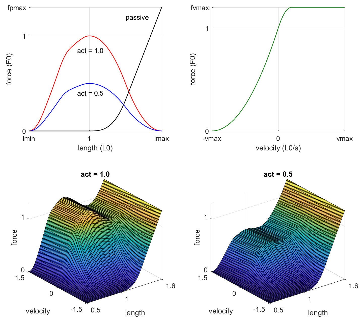
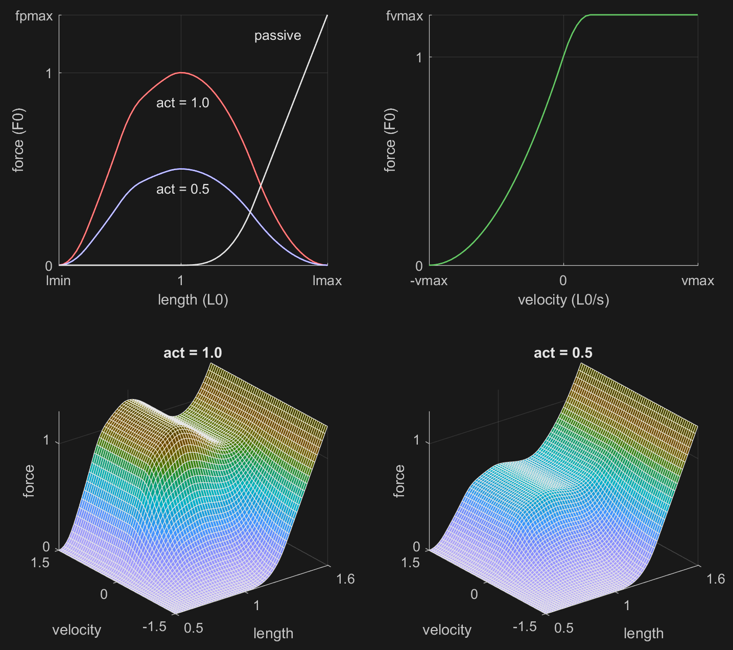
The function is in the form:

\[\text{\small FLV}(L, V, \texttt{act}) = F_L(L)\cdot F_V(V)\cdot \texttt{act} + F_P(L) \]

Comparing to the general form of a MuJoCo actuator, we see that \(F_L\cdot F_V\) is the actuator gain and \(F_P\) is the actuator bias. \(F_L\) is the active force as a function of length, while \(F_V\) is the active force as a function of velocity. They are multiplied to obtain the overall active force (note the scaling by act which is the actuator activation). \(F_P\) is the passive force which is always present regardless of activation. The output of the \(\text{\small FLV}\) function is the scaled muscle force. We multiply the scaled force by a muscle-specific constant \(F_0\) to obtain the actual force:

\[\texttt{actuator\_force} = -\text{\small FLV}(L, V, \texttt{act}) \cdot F_0 \]

The negative sign is because positive muscle activation generates pulling force. The constant \(F_0\) is the peak active force at zero velocity. It is related to the muscle thickness (i.e., physiological cross-sectional area or PCSA). If known, it can be set with the attribute force of element muscle. If it is not known, we set it to \(-1\) which is the default. In that case we rely on the fact that larger muscles tend to act on joints that move more weight. The attribute scale defines this relationship as:

\[F_0 = \text{scale} / \texttt{actuator\_acc0} \]

The quantity \(\texttt{actuator\_acc0}\) is precomputed by the model compiler. It is the norm of the joint acceleration caused by unit force acting on the actuator transmission. Intuitively, \(\text{scale}\) determines how strong the muscle is “on average” while its actual strength depends on the geometric and inertial properties of the entire model.

Thus far we encountered three constants that define the properties of an individual muscle: \(L_T, L_0, F_0\). In addition, the function \(\text{\small FLV}\) itself has several parameters illustrated in the above figure: \(l_\text{min}, l_\text{max}, v_\text{max}, f_\text{pmax}, f_\text{vmax}\). These are supposed to be the same for all muscles, however different experimental papers suggest different shapes of the FLV function, thus users familiar with that literature may want to adjust them. We provide the MATLAB function FLV.m which was used to generate the above figure and shows how we compute the \(\text{\small FLV}\) function.

Before embarking on a mission to design more accurate \(\text{\small FLV}\) functions, consider the fact that the operating range of the muscle has a bigger effect than the shape of the \(\text{\small FLV}\) function, and in many cases this parameter is unknown. Below is a graphical illustration:

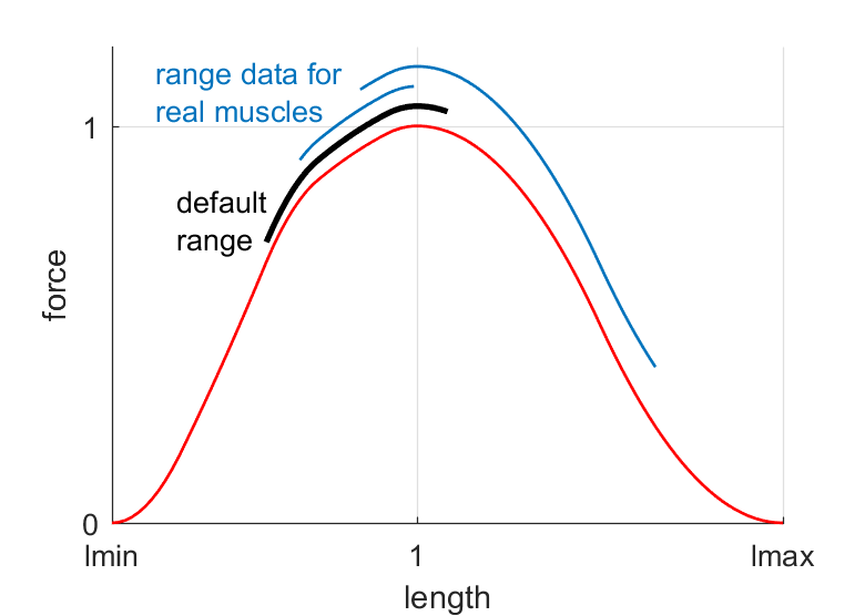
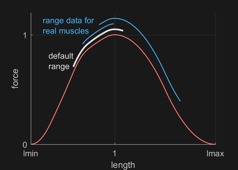
This figure format is common in the biomechanics literature, showing the operating range of each muscle superimposed on the normalized \(\text{FL}\) curve (ignore the vertical displacement). Our default range is shown in black. The blue curves are experimental data for two arm muscles. One can find muscles with small range, large range, range spanning the ascending portion of the \(\text{FL}\) curve, or the descending portion, or some of both. Now suppose you have a model with 50 muscles. Do you believe that someone did careful experiments and measured the operating range for every muscle in your model, taking into account all the joints that the muscle spans? If not, then it is better to think of musculo-skeletal models as having the same general behavior as the biological system, while being different in various details – including details that are of great interest to some research community. For most muscle properties which modelers consider constant and known, there is an experimental paper showing that they vary under some conditions. This is not to discourage people from building accurate models, but rather to discourage people from believing too strongly in their models.

Coming back to our muscle model, there is the muscle activation act. This is the state of a first-order nonlinear filter whose input is the control signal. The filter dynamics are:

\[\frac{\partial}{\partial t}\texttt{act} = \frac{\texttt{ctrl} - \texttt{act}}{\tau(\texttt{ctrl}, \texttt{act})} \]

Internally the control signal is clamped to [0, 1] even if the actuator does not have a control range specified. There are two time constants specified with the attribute timeconst, namely \(\text{timeconst} = (\tau_\text{act}, \tau_\text{deact})\) with defaults \((0.01, 0.04)\). Following Millard et al. (2013), the effective time constant \(\tau\) is then computed at runtime as:

\[\tau(\texttt{ctrl}, \texttt{act}) = \begin{cases} \tau_\text{act} \cdot (0.5 + 1.5\cdot\texttt{act}) & \texttt{ctrl}-\texttt{act} \gt 0 \\ \tau_\text{deact} / (0.5 + 1.5\cdot\texttt{act}) & \texttt{ctrl} - \texttt{act} \leq 0 \end{cases} \]

Since the above equation describes discontinuous switching, which can be undesirable when using derivative-based optimization, we introduce the optional smoothing parameter tausmooth. When greater than 0, the switching is replaced by mju_sigmoid, which will smoothly interpolate between the two values within the range \((\texttt{ctrl}-\texttt{act}) \pm \text{tausmooth}/2\).

Now we summarize the attributes of element muscle which users may want to adjust, depending on their familiarity with the biomechanics literature and availability of detailed measurements with regard to a particular model:

Defaults

Use the built-in defaults everywhere. All you have to do is attach a muscle to a tendon, as shown at the beginning of this section. This yields a generic yet reasonable model.

scale

If you do not know the strength of individual muscles but want to make all muscles stronger or weaker, adjust scale. This can be adjusted separately for each muscle, but it makes more sense to set it once in the default element.

force

If you know the peak active force \(F_0\) of the individual muscles, enter it here. Many experimental papers contain this data.

range

The operating range of the muscle in scaled lengths is also available in some papers. It is not clear how reliable such measurements are (given that muscles act on many joints) but they do exist. Note that the range differs substantially between muscles.

timeconst

Muscles are composed of slow-twitch and fast-twitch fibers. The typical muscle is mixed, but some muscles have a higher proportion of one or the other fiber type, making them faster or slower. This can be modeled by adjusting the time constants. The vmax parameter of the \(\text{\small FLV}\) function should also be adjusted accordingly.

tausmooth

When positive, smooths the transition between activation and de-activation time-constants. While a single motor unit is either activating or de-activating, an entire muscle will have a mixture of many units, leading to a corresponding mixture of timescales.

lmin, lmax, vmax, fpmax, fvmax

These are the parameters controlling the shape of the \(\text{\small FLV}\) function. Advanced users can experiment with them; see MATLAB function FLV.m. Similar to the scale setting, if you want to change the \(\text{\small FLV}\) parameters for all muscles, do so in the default element.

Custom model

Instead of adjusting the parameters of our muscle model, users can implement a different model, by setting gaintype, biastype and dyntype of a general actuator to “user” and providing callbacks at runtime. Or, leave some of these types set to “muscle” and use our model, while replacing the other components. Note that tendon geometry computations are still handled by the standard MuJoCo pipeline providing actuator_length, actuator_velocity and actuator_lengthrange as inputs to the user’s muscle model. Custom callbacks could then simulate elastic tendons or any other detail we have chosen to omit.

Relation to OpenSim

The standard software used by researchers in biomechanics is OpenSim. We have designed our muscle model to be similar to the OpenSim model where possible, while making simplifications which result in significantly faster and more stable simulations. To help MuJoCo users convert OpenSim models, here we summarize the similarities and differences.

The activation dynamics model is identical to OpenSim, including the default time constants.

The \(\text{\small FLV}\) function is not exactly the same, but both MuJoCo and OpenSim approximate the same experimental data, so they are very close. For a description of the OpenSim model and summary of relevant experimental data, see Millard et al. (2013).

We assume inelastic tendons while OpenSim can model tendon elasticity. We decided not to do that here, because tendon elasticity requires fast-equilibrium assumptions which in turn require various tweaks and are prone to simulation instability. In practice tendons are quite stiff, and their effect can be captured approximately by stretching the \(\text{FL}\) curve corresponding to the inelastic case (Zajac (1989)). This can be done in MuJoCo by shortening the muscle operating range.

Pennation angle (i.e., the angle between the muscle and the line of force) is not modeled in MuJoCo and is assumed to be 0. This effect can be approximated by scaling down the muscle force and also adjusting the operating range.

Tendon wrapping is also more limited in MuJoCo. We allow spheres and infinite cylinders as wrapping objects, and require two wrapping objects to be separated by a fixed site in the tendon path. This is to avoid the need for iterative computations of tendon paths. We also allow “side sites” to be placed inside the sphere or cylinder, which causes an inverse wrap: the tendon path is constrained to pass through the object instead of going around it. This can replace torus wrapping objects used in OpenSim to keep the tendon path within a given area. Overall, tendon wrapping is the most challenging part of converting an OpenSim model to a MuJoCo model, and requires some manual work. On the bright side, there is a small number of high-quality OpenSim models in use, so once they are converted we are done.

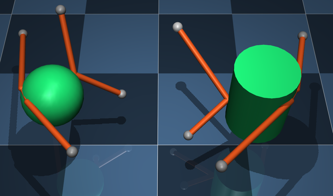
Below we illustrate the four types of tendon wrapping available. Note that the curved sections of the wrapping tendons are rendered as straight, but the geometry pipeline works with the actual curves and computes their lengths and moments analytically:

Sensors

MuJoCo can simulate a wide variety of sensors as described in the sensor element below. User sensor types can also be defined, and are evaluated by the callback mjcb_sensor. Sensors do not affect the simulation. Instead their outputs are copied in the array mjData.sensordata and are available for user processing.

Here we describe the XML attributes common to all sensor types, so as to avoid repetition later.

name: string, optional

Name of the sensor.

noise: real, “0”

The standard deviation of the noise model of this sensor. In versions prior to 3.1.4, this would lead to noise being added to the sensors. In release 3.1.4 this feature was removed, see 3.1.4 changelog for a detailed justification. As of subsequent versions, this attrbute serves as a convenient location for saving standard deviation information for later use.

cutoff: real, “0”

When this value is positive, it limits the absolute value of the sensor output. It is also used to normalize the sensor output in the sensor data plots in simulate.cc.

user: real(nuser_sensor), “0 0 …”

See User parameters.

Cameras

Besides the default, user-controllable, free camera, “fixed” cameras can be attached to the kinematic tree.

Extrinsics

By default, camera frames are attached to the containing body. The optional mode and target attributes can be used to specify camera that track (move with) or target (look at) a body or subtree. Cameras look towards the negative Z axis of the camera frame, while positive X and Y correspond to right and up in the image plane, respectively.

Intrinsics

Camera intrinsics are specified using ipd (inter-pupilary distance, required for stereoscopic rendering and VR) and fovy (vertical field of view, in degrees).

The above specification implies a perfect point camera with no aberrations. However when calibrating real cameras, two types of linear aberration can be expressed using standard rendering pipelines. The first is different focal lengths in the vertical and horizontal directions (axis-aligned astigmatism). The second is a non-centered principal point. These can be specified using the focal and principal attributes. When these calibration-related attributes are used, the physical sensor size and camera resolution must also be specified. In this case, the rendering frustum can be visualized.

Composite objects

Composite objects are not new model elements. Instead, they are (large) collections of existing elements designed to simulate particle systems, ropes, cloth, and soft bodies. These collections are generated by the model compiler automatically. The user configures the automatic generator on a high level, using the new XML element composite and its attributes and sub-elements, as described in the XML reference chapter. If the compiled model is then saved, composite is no longer present and is replaced with the collection of regular model elements that were automatically generated. So think of it as a macro that gets expanded by the model compiler.

Composite objects are made up of regular MuJoCo bodies, which we call “element bodies” in this context. The element bodies are created as children of the body within which composite appears; thus a composite object appears in the same place in the XML where a regular child body may have been defined. Each automatically-generated element body has a single geom attached to it, usually a sphere but could also be a capsule or an ellipsoid. Thus the composite object is essentially a particle system, however the particles can be constrained to move together in ways that simulate various flexible objects. The initial positions of the element bodies form a regular grid in 1D, 2D or 3D. They could all be children of the parent body (which can be the world or another regular body; composite objects cannot be nested) and have joints allowing motion relative to the parent, or they could form a kinematic tree with joints between the element bodies. They can also be connected with tendons with soft equality constraints on the tendon length, creating the necessary coupling. Joint equality constraints are also used in some cases. The solref and solimp attributes of these equality constraints can be adjusted by the user, thereby adjusting the softness and flexibility of the composite objects.

In addition to setting up the physics, the composite object generator creates suitable rendering. 2D and 3D objects can be rendered as skins. The skin is generated automatically, and can be textured as well as subdivided using bi-cubic interpolation. The actual physics and in particular the collision detection are based on the element bodies and their geoms, while the skin is purely a visualization object. Yet in most situations we prefer to look at the skin representation. To facilitate this, the generator places all geoms, sites and tendons in group 3 whose visualization is disabled by default. So when you load a 2D grid for example, you will see a continuous flexible surface and not a collection of spheres connected with tendons. However when fine-tuning the model and trying to understand the physics behind it, it is useful to be able to render the spheres and tendons. To switch the rendering style, disable the rendering of skins and enable group 3 for geoms and tendons.

We have designed the composite object generator to have intuitive high-level controls as much as possible, but at the same time it exposes a large number of options that interact with each other and can profoundly affect the resulting physics. So at some point users should read the reference documentation carefully. As a quick start though, MuJoCo comes with an example of each composite object type. Below we go over these examples and explain the less obvious aspects. In all examples we have a static scene which is included in the model, followed by a single composite object. The static scene has a mocap body (large capsule) that can be moved around with the mouse to probe the behavior of the system. The XML snippets below are just the definition of the composite object; see the XML model files in the distribution for the complete examples.

Particle.

<worldbody>
  <composite type="particle" count="10 10 10" spacing="0.07" offset="0 0 1">
    <geom size=".02" rgba=".8 .2 .1 1"/>
  </composite>
</worldbody>

The above XML is all it takes to create a system with 1000 particles with initial positions on a 10-10-10 grid, and set the size, color, spacing and offset of the particles. The resulting element bodies become children of the world body. One could adjust many other properties including the softness of the contacts and the joint attributes. The plot on the right shows the joints. Each element body has 3 orthogonal slider joints, allowing it to translate but not rotate. The idea is that particles should have position but no orientation. MuJoCo bodies always have orientation, however by using only slider joints we do not allow the orientation to change. The geom defaults are adjusted automatically so that they make frictionless contacts with each other and with the rest of the model. So this system has 1000 bodies (each with a geom), 3000 degrees of freedom and around 1000 active contacts. Evaluating the dynamics takes around 1 ms on a single core of a modern processor. As with most other MuJoCo models, the soft constraints allow simulation at much larger timesteps (this model is stable at 30 ms timestep and even higher).

Particles are also compatible with the passive forces 2D and 3D plugins, discussed in the deformable section. However, collisions are limited to the particle themselves and not to the whole boundary of the skin that encloses them. This makes contacts very fast but does not guarantee that all penetrations can be avoided. For a more complete treatment, see again the deformable section, which outlines how to use flexcomp to create such an object. It is easy to port models create with composite particles to flex, see the folder elasticity/ for several examples.

1D grid.

<composite type="grid" count="20 1 1" spacing="0.045" offset="0 0 1">
  <joint kind="main" damping="0.001"/>
  <tendon kind="main" width="0.01"/>
  <geom size=".02" rgba=".8 .2 .1 1"/>
  <pin coord="1"/>
  <pin coord="13"/>
</composite>

The grid type can create 1D or 2D grids, depending on the count attribute. Here we illustrate 1D grids. These are strings of spheres connected with tendons whose length is soft-equality-constrained. The softness can be adjusted. Similar to particles, the element bodies here have slider joints but no rotational joints. The plot on the right illustrates pinning. The pin sub-element is used to specify the grid coordinates of the pinned bodies, and the model compiler does not generate joints for these bodies, thereby fixing them rigidly to the parent body (in this case the world). This makes the string in the right plot hang in space. The same mechanism can be used to model a whip for example; in that case the parent body would be moving, and the first element body would be pinned to the parent.

2D grid.

<composite type="grid" count="9 9 1" spacing="0.05" offset="0 0 1">
  <skin material="matcarpet" inflate="0.001" subgrid="3" texcoord="true"/>
  <geom size=".02"/>
  <pin coord="0 0"/>
  <pin coord="8 0"/>
</composite>

A 2D grid can be used to simulate cloth. What it really simulates is a 2D grid of spheres connected with equality-constrained tendons (not shown). The model compiler can also generate skin, enabled with the skin sub-element in the above XML. Some of the element bodies can also be pinned, similar to 1D grids but using two grid coordinates. The plot on the right shows a cloth pinned to the world body at the two corners, and draping over our capsule probe. The skin on the right is subdivided using bi-cubic interpolation, which increases visual quality in the absence of textures. When textures are present (left) the benefits of subdivision are less visible.

Cable.

<extension>
   <plugin plugin="mujoco.elasticity.cable"/>
</extension>

<worldbody>
   <composite prefix="actuated" type="cable" curve="cos(s) sin(s) s" count="41 1 1"
              size="0.25 .1 4" offset="0.25 0 .05" initial="none">
      <plugin plugin="mujoco.elasticity.cable">
         <!--Units are in Pa (SI)-->
         <config key="twist" value="5e8"/>
         <config key="bend" value="15e8"/>
         <config key="vmax" value="0"/>
      </plugin>
      <joint kind="main" damping="0.15" armature="0.01"/>
      <geom type="capsule" size=".005" rgba=".8 .2 .1 1"/>
   </composite>
</worldbody>

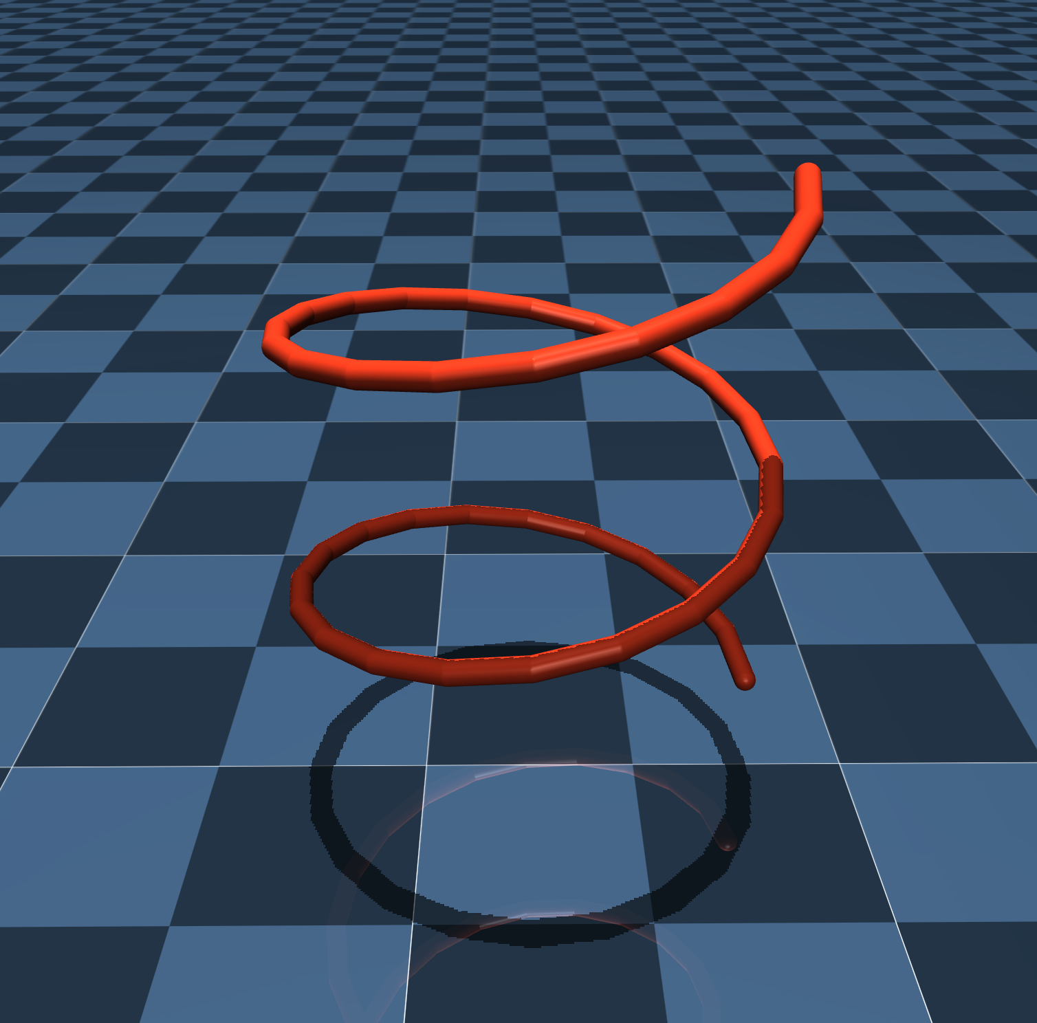
The cable simulates an inextensible elastic 1D object having twist and bending stiffness. It is discretized using a sequence of capsules or boxes. Its stiffness and inertia properties are computed directly from the given parameters and the shape of the cross section, which allows for anisotropic behaviors, which can be found in e.g. belts or computer cables. It is a single kinematic tree, so it is exactly inextensible without the use of additional constraints, enabling the use of large time steps. The elastic model is geometrically exact and based on computing the Bishop or twist-free frame of the centerline, i.e., the line passing through the center of the cross section. The orientations of the geoms are expressed with respect to this frame and then decomposed into twist and bending components, hence different stiffnesses can be set independently. Moreover, it is possible to specify if the stress-free configuration is flat or curve, such as in the case of coil springs. The cable requires using a first-party engine plugin, which may be integrated directly into the engine in the future.

Rope and loop.

The rope and loop are deprecated. It is recommended to use the cable for simulating inextensible elastic rods that are bent and twisted and 1D flex deformable objects for extensible strings in a tensile loading scenario (e.g. a stretched rubber band).

Cloth.

The cloth is deprecated. It is recommended to use 2D flex deformable objects for simulating thin elastic structures.

Box.

<body pos="0 0 1">
  <freejoint/>
  <composite type="box" count="7 7 7" spacing="0.04">
    <skin texcoord="true" material="matsponge" rgba=".7 .7 .7 1"/>
    <geom type="capsule" size=".015 0.05" rgba=".8 .2 .1 1"/>
  </composite>
</body>

The box type, as well as the cylinder and ellipsoid types below, are used to model soft 3D objects. The element bodies form a grid along the outer shell, thus the number of element bodies scales with the square of the linear dimension. This is much more efficient than simulating a 3D grid. The parent body within which composite appears is at the center of the soft object. All element bodies are children of the parent. Each element body has a single sliding joint pointing away from the parent. These joints allow the surface of the soft object to compress and expand at any point. The joints are equality-constrained to their initial position, so as to maintain the shape. In addition each joint is equality-constrained to its neighbor joints, so that when the soft objects deforms, the deformation is smooth. Finally, there is a tendon equality constraint specifying that the sum of all joints should remain constant. This attempts to preserve the volume of the soft object approximately. If the object is squeezed from all sides it will compress and the volume will decrease, but otherwise some element bodies will stick out to compensate for squeezing elsewhere. The plot on the left shows this effect; we are using the capsule probe to compress one corner, and the opposite sides of the cube expand a bit, while the deformations remain smooth. The count attribute determines the number of element bodies in each dimension, so if the counts are different the resulting object will be a rectangular box and not a cube. The geoms attached to the element bodies can be spheres, capsules or ellipsoids. Spheres are faster for collision detection, but they result in a thin shell, allowing other bodies to “get under the skin” of the soft object. When capsules or ellipsoids are used, they are automatically oriented so that the long axis points to the outside, thus creating a thicker shell which is harder to penetrate.

Cylinder and ellipsoid.

<body pos="0 0 1">
  <freejoint/>
  <composite type="ellipsoid" count="5 7 9" spacing="0.05">
    <skin texcoord="true" material="matsponge" rgba=".7 .7 .7 1"/>
    <geom type="capsule" size=".015 0.05" rgba=".8 .2 .1 1"/>
  </composite>
</body>

Cylinders and ellipsoids are created in the same way as boxes. The only difference is that the reference positions of the element bodies (relative to the parent) are projected on a cylinder or ellipsoid, with size implied by the count attribute. The automatic skin generator is aware of the smooth surfaces, and adjusts the skin normals accordingly. In the plots we have used the capsule probe to press on each body, then paused the simulation and moved the probe away (which is possible because the probe is a mocap body which can move independent of the physics). In this way we can see the indentation made by the probe, and the resulting deformation in the rest of the body. By changing the solref and solimp attributes of the equality constraints that hold the soft object together, one can adjust the behavior of the system making it softer or harder, damped or springy, etc. Note that box, cylinder and ellipsoid objects do not involve long kinematic chains, and can be simulated at large timesteps - similar to particle and grid, and unlike rope and cloth.

Deformable objects

The composite objects described earlier were intended to emulate soft bodies in what is effectively a rigid-body simulator. This was possible because MuJoCo constraints are soft, but nevertheless it was limited in functionality and modeling power. In MuJoCo 3.0 we have introduced true deformable objects involving new model elements. The skin described earlier was actually one such element, but it is merely used for visualization. We now have a related element flex which generates contact forces, constraint forces and passive forces as needed to model a wide range of deformable entities. Both skins and flexes are now defined within a new grouping element in the XML called deformable. A flex is a low-level element that specifies everything needed at runtime, but is difficult to design at modeling time. To aid with modeling, we have further introduced the element flexcomp which automates the creation of the low-level flex, similar to how composite automates the creation of (collections of) MuJoCo objects needed to emulate a soft body. Flexes may eventually supersede composites, but for now both are useful for somewhat different purposes.

A flex is a collection of MuJoCo bodies that are connected with massless stretchable elements. These elements can be capsules (1D flex), triangles (2D flex), or tetrahedra (3D flex). In all cases we allow a radius, which makes the elements smooth and also volumetric in 1D and 2D. The primitive elements are illustrated below:

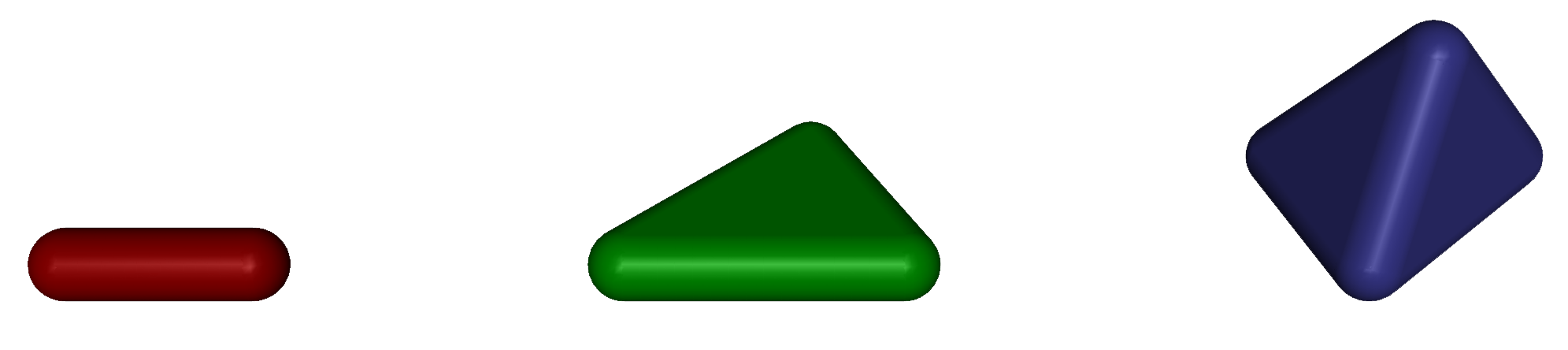
Thus far these look like geoms. But the key difference is that they deform: as the bodies (vertices) move independently of each other, the shape of the elements changes in real time. Collisions and contact forces are now generalized to handle these deformable geometric elements. Note that when two such elements collide, the contact no longer involves just two bodies, but can involve up to 8 bodies (if both elements are tetrahedra). Contact forces are computed as before, given the contact frame and relevant quantities expressed in that frame. But then the contact force is distributed among all interacting bodies. The notion of contact Jacobian is complicated because the contact point cannot be considered fixed in any body frame. Instead we use a weighting scheme to “assign” each contact point to multiple bodies. It is also possible to create a rigid flex, by assigning all vertices to the same body. This is a way to re-purpose the new flex collision machinery to implement rigid non-convex mesh collisions (unlike mesh geoms which are convexified for collision purposes).

Deformation model.

In order to preserve the shape of the flex (in a soft sense), we need to generate passive or constraint forces. Prior to MuJoCo 3.0 this would involve a large number of tendons plus constraints on tendons and joints. This is still possible here, but inefficient both in terms of modeling and in terms of simulation when the flex is large. Instead, the design philosophy is to use a single set of parameters and provide two modeling choices: a new (soft) equality constraint type that applies to all edges of a given flex, which permits large time steps, or a discretized continuum representation, where each element is in a constant stress state, which is equivalent to piecewise linear finite elements and achieves improved realism and accuracy. The edge-based model could be seen as a “lumped” stiffness model, where the correct coupling of deformation modes (e.g. shear and volumetric) is averaged in a single quantity. The continuum model enables instead to specify shear and volumetic stiffnesses separately using the Poisson’s ratio of the material. For more details, see the Saint Venant-Kirchhoff hyperelastic model. This functionality is currently based on first-party engine plugins as of MuJoCo 3.0 but may be integrated into the engine in future releases.

Creation and visualization.

<option timestep=".001"/>

<extension>
   <plugin plugin="mujoco.elasticity.solid"/>
</extension>

<worldbody>
   <flexcomp type="grid" count="24 4 4" spacing=".1 .1 .1" pos=".1 0 1.5"
             radius=".0" rgba="0 .7 .7 1" name="softbody" dim="3" mass="7">
      <contact condim="3" solref="0.01 1" solimp=".95 .99 .0001" selfcollide="none"/>
      <edge damping="1"/>
      <plugin plugin="mujoco.elasticity.solid">
         <config key="poisson" value="0.2"/>
         <!--Units are in Pa (SI)-->
         <config key="young" value="5e4"/>
      </plugin>
   </flexcomp>
</worldbody>

Using the flexcomp element, we can create flexes from meshes, including tetrahedral meshes, and automatically generate all the bodies/vertices and connect them with suitable elements. We can also create grids and other topologies automatically. This machinery makes it easy to create very large flexes, involving thousands or even tens of thousands of bodies, elements and edges. Obviously such simulations will not be fast. Even for medium-sized flexes, pruning of collision pairs and essential. This is why we have developed elaborate methods for pruning self-collisions; see XML reference.

In case of 3D flexes made of tetrahedra, it may be useful to examine how the flex is “triangulated” internally. We have a special visualization mode that peels off the outer layers. Below is an example with the Stanford Bunny. Note how it has smaller tetrahedra on the outside and larger ones on the inside. This mesh design makes sense, because we want the collision surface to be accurate, but on the inside we just need soft material properties - which require less spatial resolution. In order to convert a surface mesh to a tetrahedral mesh, we recommend open tools like the fTetWild library.

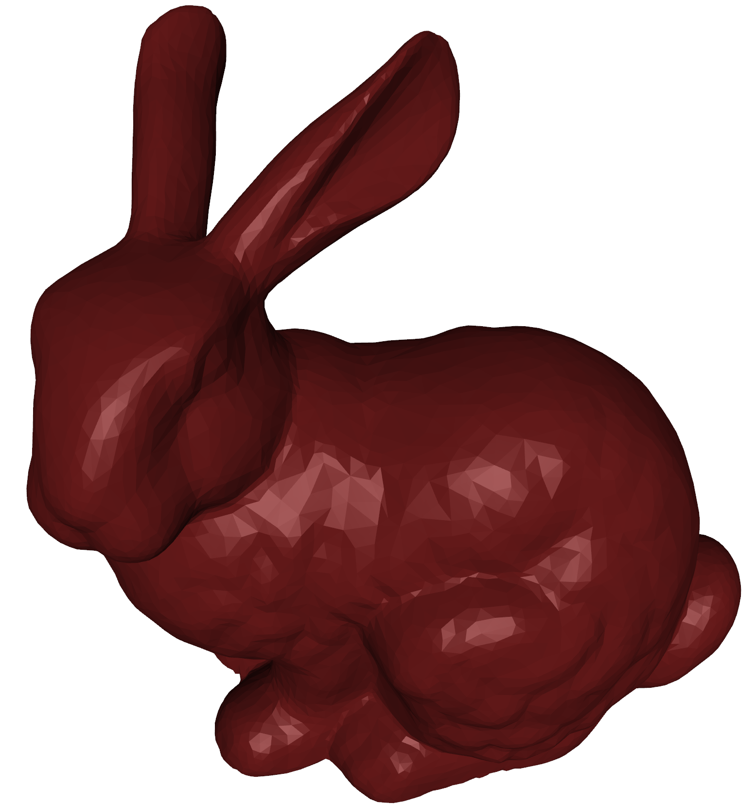
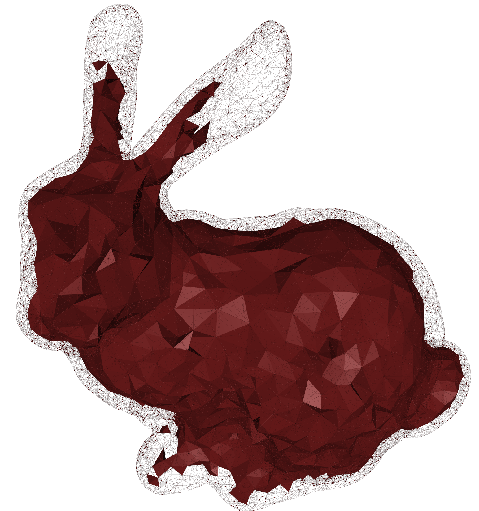
Including files

MJCF files can include other XML files using the include element. Mechanistically, the parser replaces the DOM node corresponding to the include element in the master file with the list of XML elements that are children of the top-level element in the included file. The top-level element itself is discarded, because it is a grouping element for XML purposes and would violate the MJCF format if included.

This functionality enables modular MJCF models; see the MPL family of models in the model library. One example of modularity is constructing a model of a robot (which tends to be elaborate) and then including it in multiple “scenes”, i.e., MJCF models defining the objects in the robot’s environment. Another example is creating a file with commonly used assets (say materials with carefully adjusted rgba values) and including it in multiple models which reference those assets.

The included files are not required to be valid MJCF files on their own, but they usually are. Indeed we have designed this mechanism to allow MJCF models to be included in other MJCF models. To make this possible, repeated MJCF sections are allowed even when that does not make sense semantically in the context of a single model. For example, we allow the kinematic tree to have multiple roots (i.e., multiple worldbody elements) which are merged automatically by the parser. Otherwise including robots into scenes would be impossible.

The flexibility of repeated MCJF sections comes at a price: global settings that apply to the entire model, such as the angle attribute of compiler for example, can be defined multiple times. MuJoCo allows this, and uses the last definition encountered in the composite model, after all include elements have been processed. So if model A is defined in degrees and model B is defined in radians, and A is included in B after the compiler element in B, the entire composite model will be treated as if it was defined in degrees - leading to undesirable consequences in this case. The user has to make sure that models included in each other are compatible in this sense; local vs. global coordinates is another compatibility requirement.

Finally, as explained next, element names must be unique among all elements of the same type. So for example if the same geom name is used in two models, and one model is included in the other, this will result in compile error. Including the same XML file more than once is a parsing error. The reason for this restriction is that we want to avoid repeated element names as well as infinite recursion caused by inclusion.

Naming elements

Most model elements in MJCF can have names. They are defined with the attribute name of the corresponding XML element. When a given model element is named, its name must be unique among all elements of the same type. Names are case-sensitive. They are used at compile time to reference the corresponding element, and are also saved in mjModel for user convenience at runtime.

The name is usually an optional attribute. We recommend leaving it undefined (so as to keep the model file shorter) unless there is a specific reason to define it. There can be several such reasons:

• Some model elements need to reference other elements as part of their creation. For example, a spatial tendon needs to reference sites in order to specify the via points it passes through. Referencing can only be done by name. Note that assets exist for the sole purpose of being referenced, so they must have a name, however it can be omitted and set implicitly from the corresponding file name.

• The visualizer offers the option to label all model elements of a given type. When a name is available, it is printed next to the object in the 3D view; otherwise a generic label in the format “body 7” is printed.

• The function mj_name2id returns the index of the model element with given type and name. Conversely, the function mj_id2name returns the name given the index. This is useful for custom computations involving a model element that is identified by its name in the XML (as opposed to relying on a fixed index which can change when the model is edited).

• The model file could in principle become more readable by naming certain elements. Keep in mind however that XML itself has a commenting mechanism, and that mechanism is more suitable for achieving readability - especially since most text editors provide syntax highlighting which detects XML comments.

URDF extensions

The Unified Robot Description Format (URDF) is a popular XML file format in which many existing robots have been modeled. This is why we have implemented support for URDF even though it can only represent a subset of the model elements available in MuJoCo. In addition to standard URDF files, MuJoCo can load files that have a custom (from the viewpoint of URDF) mujoco element as a child of the top-level element robot. This custom element can have sub-elements compiler, option, size with the same functionality as in MJCF, except that the default compiler settings are modified so as to accomodate the URDF modeling convention. The compiler extension in particular has proven very useful, and indeed several of its attributes were introduced because a number of existing URDF models have non-physical dynamics parameters which MuJoCo’s built-in compiler will reject if left unmodified. This extension is also needed to specify mesh directories.

Note that the while MJCF models are checked against a custom XML schema by the parser, URDF models are not. Even the MuJoCo-specific elements embedded in the URDF file are not checked. As a result, mis-typed attribute names are silently ignored, which can result in major confusion if the typo remains unnoticed.

Here is an example extension section of a URDF model:

<robot name="darwin">
  <mujoco>
    <compiler meshdir="../mesh/darwin/" balanceinertia="true" discardvisual="false"/>
  </mujoco>
  <link name="MP_BODY">
    ...
</robot>

The above extensions make URDF more usable but still limited. If the user wants to build models taking full advantage of MuJoCo and at the same time maintain URDF compatibility, we recommend the following procedure. Introduce extensions in the URDF as needed, load it and save it as MJCF. Then add information to the MJCF using include elements whenever possible. In this way, if the URDF is modified, the corresponding MJCF can be easily re-created. In our experience though, URDF files tend to be static while MJCF files are often edited. Thus in practice it is usually sufficient to convert the URDF to MJCF once and after that only work with the MJCF.

MoCap bodies

mocap bodies are static children of the world (i.e., have no joints) and their mocap attribute is set to “true”. They can be used to input a data stream from a motion capture device into a MuJoCo simulation. Suppose you are holding a VR controller, or an object instrumented with motion capture markers (e.g. Vicon), and want to have a simulated object moving in the same way but also interacting with other simulated objects. There is a dilemma here: virtual objects cannot push on your physical hand, so your hand (and thereby the object you are controlling) can violate the simulated physics. But at the same time we want the resulting simulation to be reasonable. How do we do this?

The first step is to define a mocap body in the MJCF model, and implement code that reads the data stream at runtime and sets mjModel.mocap_pos and mjModel.mocap_quat to the position and orientation received from the motion capture system. The simulate.cc code sample uses the mouse as a motion capture device, allowing the user to move mocap bodies around:

The key thing to understand about mocap bodies is that the simulator treats them as being fixed. We are causing them to move from one simulation time step to the next by updating their position and orientation directly, but as far as the physics model is concerned their position and orientation are constant. So what happens if we make contact with a regular dynamic body, as in the composite object examples provided with the MuJoCo distribution (recall that in those example we have a capsule probe which is a mocap body that we move with the mouse). A contact between two regular bodies will experience penetration as well as relative velocity, while contact with a mocap body is missing the relative velocity component because the simulator does not know that the mocap body itself is moving. So the resulting contact force is smaller and it takes longer for the contact to push the dynamic object away. Also, in more complex simulations the fact that we are doing something inconsistent with the physics can cause instabilities.

There is however a better-behaved alternative. In addition to the mocap body, we include a second regular body and connect it to the mocap body with a weld equality constraint. In the plots below, the pink box is the mocap body and it is connected to the base of the hand. In the absence of other constraints, the hand tracks the mocap body almost perfectly (and much better than a spring-damper would) because the constraints are handled implicitly and can produce large forces without destabilizing the simulation. But if the hand is forced to make contact with the table for example (right plot) it cannot simultaneously respect the contact constraint and track the mocap body. This is because the mocap body is free to go through the table. So which constraint wins? That depends on the softness of the weld constraint realtive to the contact constraint. The corresponding solref and solimp parameters need to be adjusted so as to achieve the desired trade-off. See the Modular Prosthetic Limb (MPL) hand model available on the MuJoCo Forum for an example; the plots below are generated with that model.

Memory allocation

MuJoCo preallocates all the memory needed at runtime in mjData, and does not access the heap allocator after model creation. Memory in mjData is allocated by mj_makeData in two contiguous blocks:

• mjData.buffer contains fixed-size arrays.

• mjData.arena contains dynamically-sized arrays.

There are two types of dynamic arrays allocated in the arena memory space.

• contacts and constraint-related arrays are laid out from the beginning of the arena.

• stack arrays are laid out from the end of the arena.

By allocating dynamic quantities from both sides of the arena space, variable-sized memory allocation is controlled by a single number: the memory attribute of the size MJCF element. Unlike the fixed-size arrays in the buffer, variable-sized arrays in the arena can be NULL, for example after a call to mj_resetData. When arena memory runs out, one of three things will happen, depending on the type of memory requested:

• If memory runs out during contact allocation, a warning will be raised and subsequent contacts will not be added in this step, but simulation continues as usual.

• If memory runs out during constraint-related allocation, a warning will be raised and the constraint solver will be disabled in this step, but simulation continues as usual. Note that physics without the constraint solver will generally be very different, but allowing the simulation to continue can still be useful, e.g. during scene initialization when many bodies are temporarily overlapping.

• If memory runs out during stack array allocation, a hard error will occur.

Unlike the size of the buffer, the size of the arena cannot be pre-computed, since the number of contacts and stack usage is not known in advance. So how should one choose it? The following simple heuristic is currently used, though it may be improved in the future: enough memory is allocated for 100 contacts and 500 scalar constraints, under worst-case conditions. If this heuristic is insufficient, we recommend the following procedure. Increase the arena memory significantly using the memory attribute, and inspect the actual memory used at runtime. mjData.maxuse_arena keeps track of the maximum arena memory utilization since the last reset. The simulate viewer shows this number as a fraction of the total arena space (in the info window in the lower-left corner). So one can start with a large number, simulate for a while, and if the fractions are small go back to the XML and reduce the allocation size. Keep in mind though that memory utilization can change dramatically in the course of the simulation, depending on how many constraints are active and which constraint solver is used. The CG solver is the most memory efficient, followed by the Newton solver, while the PGS solver is the most memory intensive. When we design models, we usually aim for 50% utilization in the worst-case scenario encountered while exploring the model. If you only intend to use the CG solver, you can get away with significantly smaller arena allocation.

Attention

Memory allocation behaviour changed in MuJoCo 2.3.0. Before this version, the njmax, nconmax and nstack attributes of the size MJCF element had the semantics of maximum memory allocated for contacts, constraints and stack, respectively. If you are using an earlier version of MuJoCo, please switch to an earlier documentation version to read about the previous behaviour.

Tips and tricks

Here we provide guidance on how to accomplish some common modeling tasks. There is no new material here, in the sense that everything in this section can be inferred from the rest of the documentation. Nevertheless the inference process is not always obvious, so it may be useful to have it spelled out.

Performance tuning

Here is a list of steps one can take in order to maximize simulation throughput. All of the recommendations below involve some tweaking. It is recommended that these be carried out in interactive fashion while looking at the simulate utility’s built-in profiler. A detailed and sometimes more useful profile is also reported by the testspeed utility. When embarking on the more elaborate steps below, target the most expensive pipeline component reported by the profiler. Note that some of these are subtly different for MJX, see dedicated section therein.

1. timestep: Try to increase the simulation timestep. As explained at the end of the Numerical Integration section, the timestep is the single most important parameter in any model. The default value is chosen for stability rather than efficiency, and can often be increased. At some point, increasing it further will cause diveregence, so the optimal timestep is the largest timestep at which divergence never happens or is very rare. The actual value is model-dependent.

2. integrator: Choose your integrator according to the recommendations at the end of the Numerical Integration section. The default recommended choice is the implicitfast integrator.

3. jacobian: Try switching the Jacobian setting between “dense” and “sparse”. These two options use seperate code paths using dense or sparse algebra, but are otherwise compationally identical, so the faster one is always preferred. The default “auto” heuristic does not always make the right choice.

4. Constraint solver: If the profiler reports that a large chunk of time is spent in the solver, consider the following:

   • solver: The default Newton is often the fastest solver, as it requires the smallest number of iterations to converge. For large models the CG solver might be faster, for models with more degrees of freedom than constraints, the PGS solver will be fastest, though this situation is not common.

   • iterations and tolerance: Try reducing the number of iterations or, equivalently, increasing the solver’s termination tolerance. In particular for the Newton solver, which typically acheives numerical convergence in 2-3 (expensive) iterations, the last iteration increases the precision to a level that has no noticable effect, and can be skipped.

5. Collisions: If the profiler reports that collision detection takes up a large chunk of the computation time, consider the following steps:

   • Reduce the number of checked collisions using the contype / conaffinity mechanism described in the Collison detection section.

   • Modify collision geometries, replacing expensive collision tests (e.g. mesh-mesh) with cheaper primitive-primitive collisions. As a rule of thumb, collisions which have custom pair functions in the collision table at the top of engine_collision_driver.c are significantly cheaper than those that use the generic convex-convex collider mjc_Convex. The most expensive collisions are those involving SDF geometries.

   • If replacing collision meshes with primitives is not feasible, decimate the meshes as much as possible. Open source tools like trimesh, Blender, MeshLab and CoACD are very useful in this regard.

Backlash

Backlash is present in many robotic joints. It is usually caused by small gaps between gears in the gearbox, but could also be caused by some sloppiness in the joint mechanism. The effect is that the motor can turn for a small angle before the joint turns, or vice versa (when external force is applied on the joint). Backlash can be modeled in MuJoCo as follows. Instead of having a single hinge joint within the body, define two hinge joints with identical position and orientation:

<body>
  <joint name="J1" type="hinge" pos="0 0 0" axis="0 0 1" armature="0.01"/>
  <joint name="J2" type="hinge" pos="0 0 0" axis="0 0 1" limited="true" range="-1 1"/>
</body>

Thus the overall rotation of the body relative to its parent is J1+J2. Now define an actuator acting only on J1. The small joint range on J2 keeps it near 0, yet allows it to move a bit in the direction of the force acting on it, producing a backlash effect. Note the armature attribute in J1. Without it the joint-space inertia matrix will be singular, because the two joints could accelerate in opposite directions without encountering any inertia. The physical gears responsible for the backlash actually have rotational inertia (which we call armature) so this is a realistic modeling approach. The numbers in this example should be adjusted to obtain the desired behavior. The solref and solimp parameters of the joint limit constraint could also be adjusted, to make the backlash rotation end at a softer or a harder limit.

Instead of specifying joint limits in J2, one can specify a soft equality constraint keeping J2=0. The constraint impedance function should then be adjusted so the constraint is weak near J2=0 and gets stronger away from 0. The new parameterization of impedance functions shown in Solver parameters enables this. Compared to joint limits, the equality constraint approach will generate a softer transition between the backlash regime and the limit regime. It will also be active all the time, which is convenient in user code that needs the constraint violation or constraint force as input.

Damping

Damping generates a force proportional to velocity and opposite to it. In a physical system damping always increases stability. But this is only because the Universe is equipped with an ideal continuous-time integrator which does not accumulate errors due to time discretization. In a computer simulation where time is discretized, large damping can destabilize the system because of integration errors. This was already discussed in the Computation chapter.

The standard approach to reducing integration errors is to reduce the timestep or use the Runge-Kutta integrator, both of which are effective but slow down the simulation. An alternative approach is to put all damping in the joints and use the Euler integrator. In that case damping forces are integrated implicitly - meaning that the inertia matrix is adjusted and re-factorized internally as part of the velocity update, in a way transparent to the user. Implicit integration is much more stable than explicit integration, allowing substantially larger time steps. Note that the Runge-Kutta integrator is explicit, and so is Euler except for the way it treats damping forces. Ideally we would have a fully implicit integrator, but there is no publicly available physics engine that currently has such an integrator. It is on our todo list for a future MuJoCo release.

Given this state of affairs, joint damping is better behaved than damping in tendons or actuators, because the latter are not integrated implicitly. Now consider a velocity servo producing force:

force = gain * (desired_velocity - current_velocity)

This can be modeled as a velocity actuator, however such an actuator adds damping to the system and could cause instability when the gain is high. Instead we could split the above force in two terms. For the first term, define a motor which generates force = gain * desired_velocity, by treating desired_velocity as the control signal. For the second term, add damping in the joint, with damping coefficient equal to the above servo gain. Now the overall force is the same yet the damping component of the force is integrated implicitly.

Restitution

Another mechanism exists for specifying solref, as explained in Solver parameters. When both numbers are non-positive, they are interpreted as (-stiffness, -damping) and scaled by the constraint impedance. To achieve perfect restitution for contacts and other constraints, set stiffness to some reasonably large value and damping to zero. Below is an example of a sphere bouncing on a plane with restitution coefficient of 1, so that the energy before and after contact is approximately preserved. It is not exactly preserved because the contact itself is soft and takes several time steps, and the (implicit) deformations during those time steps are not exactly energy-preserving. But the overall effect is that the ball bounces for a very long time without changing its peak height in a visible way, and the energy fluctuates around the initial value instead of drifting.

<worldbody>
  <geom type="plane" size="1 1 .1"/>

  <body pos="0 0 1">
    <freejoint/>
    <geom type="sphere" size="0.1" solref="-1000 0"/>
  </body>
</worldbody>